Lie Theory: An Intuitive Introduction for Optimization and Robotics

2026-08-06 · about 8 min read · Yufeng Jin

Lie theory is the common language for carrying optimization over "curved spaces" — rotations, poses — back into ordinary vector calculus. This note walks from manifolds and tangent spaces to hat/vee and exp/log, assembles them into one optimization step on a manifold, and closes with a hand-written \(SO(3)\) code sample.

The whole story in one sentence

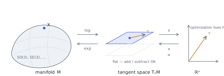
A Lie group is a "smoothly curved" space whose elements represent transformations (rotations, poses, and so on). The trouble is: you cannot add, subtract, or take gradients directly on a curved space. The fix is to shuttle back and forth between three spaces:

\[ \underbrace{\mathcal{M}}_{\text{curved manifold}} \;\xrightleftharpoons[\ \exp\ ]{\ \log\ }\; \underbrace{\mathfrak{m}}_{\text{tangent space / Lie algebra}} \;\xrightleftharpoons[\ (\cdot)^\wedge\ ]{\ (\cdot)^\vee\ }\; \underbrace{\mathbb{R}^n}_{\text{plain vector workspace}} \]

log an element down to the flat tangent space, optimize as usual in the isomorphic \(\mathbb{R}^n\), then exp it back onto the manifold. This one diagram is what the whole note is about.

A study note based on Aalok Patwardhan's A Visual Introduction to Lie Theory^[1], with the concrete derivations and code filled in.

---

Prerequisites

Prerequisites

The main text keeps returning to the following concepts, each written as an "English term = Chinese name = minimal definition" triple:

• manifold = 流形 = a smoothly curved space that looks locally like flat \(\mathbb{R}^n\) but is globally curved.^[2]
• Lie group = 李群 = an object that is both a manifold and a group whose operations (matrix multiplication and inversion) are smooth.^[4]
• tangent space = 切空间 = the flat tangent plane attached to the manifold at a given point.^[2]
• Lie algebra = 李代数 = the special tangent space of a Lie group at the identity element (written \(\mathfrak{so}(n)\) for rotation groups).^[2]
• skew-symmetric matrix = 反对称矩阵 = a matrix satisfying \(A^\top=-A\); elements of a rotation group's Lie algebra take exactly this form.^[2]
• exponential map / logarithm map = 指数映射 / 对数映射 = a pair of mutually inverse maps travelling between the tangent space and the manifold; for rotations they are the matrix exponential and matrix logarithm.^[4]

---

Problem 01 · starting point

1. Recap: optimization in Euclidean space

Start with the case where everything goes smoothly. Given a cost function \(f:\mathbb{R}^n\to\mathbb{R}\), we want the \(\mathbf{x}\) that minimizes it. The gradient descent recipe is:

1. perturb: nudge \(\mathbf{x}\) by a tiny amount;
2. gradient: compute \(\nabla f(\mathbf{x})\), which points in the direction of steepest ascent;
3. step: take a small step along \(-\nabla f\).

\[ \mathbf{x}_{k+1} = \mathbf{x}_k - \alpha\,\nabla f(\mathbf{x}_k) \]

The crucial premise here is that \(\mathbf{x}\) is a free vector. Each of its components can independently absorb a small increment \(\delta\), and the result is still a valid input. \(\mathbb{R}^n\) is "flat" and addition is unconstrained, so perturbing and stepping are entirely natural.

But what if the object being optimized is not a free vector?

Say it must be a rotation — a \(3\times3\) matrix satisfying particular constraints. Then "just perturb one number" breaks down immediately.

---

Problem 02 · the dilemma

2. The dilemma: optimizing over a rotation

Take 2D rotations as an example; the rotation matrix is:

\[ R(\theta)=\begin{bmatrix}\cos\theta & -\sin\theta\\[2pt] \sin\theta & \cos\theta\end{bmatrix} \]

It has 4 entries, but they are not free — two constraints must hold simultaneously:

\[ R^\top R = I \quad(\text{orthogonal: unit orthogonal columns}),\qquad \det R = 1\quad(\text{right-handed, no reflection}) \]

Suppose we do what we would in \(\mathbb{R}^4\) and add a small increment \(\delta\) to the top-left \(\cos\theta\):

\[ \begin{bmatrix}\cos\theta+\delta & -\sin\theta\\ \sin\theta & \cos\theta\end{bmatrix} \]

The result: it is no longer a rotation

The norm of the first column becomes \(\sqrt{(\cos\theta+\delta)^2+\sin^2\theta}\neq 1\), so \(R^\top R = I\) is violated and \(\det\) is no longer 1. You cannot "perturb one of the numbers" and keep it a rotation. The matrix entries are tightly bound together by the constraints and cannot move independently.

This is exactly where ordinary optimization hits a wall: the valid rotations do not form a flat vector space but a curved, constrained subset. Doing calculus on it requires a different toolset.

---

Concept 01 · curved spaces

3. Manifolds and Lie groups

The set of all valid 2D rotations is called the special orthogonal group \(SO(2)\); the 3D version is \(SO(3)\):

\[ SO(n)=\{\,R\in\mathbb{R}^{n\times n}\ \mid\ R^\top R=I,\ \det R = 1\,\} \]

They are manifolds: smoothly curved spaces that locally look like flat \(\mathbb{R}^n\) (much as a patch of the Earth's surface is well approximated by a flat map) but are globally curved. An object that is both a manifold and a group with smooth operations (matrix multiplication and inversion) is a Lie group^[4].

Dimension vs. degrees of freedom: why a \(3\times3\) rotation has only 3 degrees of freedom

A matrix in \(SO(3)\) has 9 entries, but \(R^\top R=I\) is a symmetric matrix equation, yielding \(\tfrac{3\cdot 4}{2}=6\) independent constraints. \(9-6=3\) ⟹ \(SO(3)\) is a 3-dimensional manifold, matching exactly the 3 degrees of freedom of "rotate by some angle about some axis". Likewise \(SO(2)\) is 1-dimensional (just the one angle \(\theta\)). This "intrinsic dimension" is precisely the number of parameters we actually want to optimize.

Figure 1. A point $X$ on a Lie group; its tangent space is a "plane" attached at that point, and that plane is in turn isomorphic to $\mathbb{R}^n$. All the optimization happens on the far right.

---

Concept 02 · tangent space

4. Lie algebra and tangent space

At a point \(X\) on the manifold, one can attach a flat tangent plane called the tangent space. The special tangent space at the identity element \(I\) is the Lie algebra of the Lie group, written \(\mathfrak{so}(n)\)^[2].

For rotations, the elements of the Lie algebra turn out to be exactly the skew-symmetric matrices (反对称矩阵, \(A^\top=-A\)):

\(\mathfrak{so}(2)\)\(\mathfrak{so}(3)\)

Only one free parameter:

\[ \boldsymbol{\theta}^\wedge=\begin{bmatrix}0 & -\theta\\ \theta & 0\end{bmatrix}=\theta\underbrace{\begin{bmatrix}0&-1\\1&0\end{bmatrix}}_{G} \]

Three free parameters \(\boldsymbol{\omega}=(\omega_1,\omega_2,\omega_3)\):

\[ \boldsymbol{\omega}^\wedge=\begin{bmatrix}0 & -\omega_3 & \omega_2\\ \omega_3 & 0 & -\omega_1\\ -\omega_2 & \omega_1 & 0\end{bmatrix} \]

It doubles as the cross-product operator: \(\boldsymbol{\omega}^\wedge\mathbf{v}=\boldsymbol{\omega}\times\mathbf{v}\).

Note that the number of independent components of a skew-symmetric matrix (1 for \(SO(2)\), 3 for \(SO(3)\)) is exactly the intrinsic dimension of the manifold. This is no accident — the dimension of the tangent space is the number of degrees of freedom. That hands us a flat, unconstrained space in which to do the math.

---

Concept 03 · proxy coordinates

5. hat and vee: \(\mathbb{R}^n\) as a proxy tangent space

The tangent space (those skew-symmetric matrices) is flat, but written as matrices it is still awkward to feed straight into an optimizer. Fortunately it is isomorphic to the ordinary vector space \(\mathbb{R}^n\) — two mutually inverse operators ferry elements between them:

• hat \((\cdot)^\wedge:\ \mathbb{R}^n\to\mathfrak{so}(n)\): lifts a workspace vector into the Lie algebra;
• vee \((\cdot)^\vee:\ \mathfrak{so}(n)\to\mathbb{R}^n\): flattens a Lie algebra element back into a workspace vector.

\[ \boldsymbol{\omega}\in\mathbb{R}^3 \ \xrightarrow{\ (\cdot)^\wedge\ }\ \boldsymbol{\omega}^\wedge\in\mathfrak{so}(3) \ \xrightarrow{\ (\cdot)^\vee\ }\ \boldsymbol{\omega}\in\mathbb{R}^3,\qquad \big((\boldsymbol{\omega}^\wedge)\big)^\vee=\boldsymbol{\omega} \]

So the object we actually hand to gradient descent is that plain 3-dimensional vector \(\boldsymbol{\omega}\) — it carries no constraints and can be perturbed however we like.

---

Concept 04 · curved to flat

6. exp and log: connecting the curved and the flat

The last piece of the puzzle is the bridge that travels between the manifold and the tangent space:

• exponential map \(\exp:\ \mathfrak{m}\to\mathcal{M}\): "wraps" an element of the tangent space back onto the curved manifold;
• logarithm map \(\log:\ \mathcal{M}\to\mathfrak{m}\): conversely, "unrolls" an element of the manifold onto the tangent space.

\[ X=\exp(\boldsymbol{\tau}^\wedge),\qquad \boldsymbol{\tau}^\wedge=\log(X) \]

For rotations, \(\exp/\log\) here are just the matrix exponential and matrix logarithm.

6.1 \(SO(2)\): transparent at a glance

Substituting \(\theta^\wedge=\theta G\) into the matrix exponential series and using \(G^2=-I\), the terms assemble themselves into \(\sin/\cos\):

\[ \exp(\theta G)=I+\theta G+\tfrac{\theta^2}{2!}G^2+\cdots =\cos\theta\,I+\sin\theta\,G =\begin{bmatrix}\cos\theta & -\sin\theta\\ \sin\theta & \cos\theta\end{bmatrix}=R(\theta) \]

Conversely \(\log R(\theta)=\theta G\), i.e. \(\theta=\operatorname{atan2}(R_{21},R_{11})\). The number \(\theta\) living in the tangent space is the rotation angle itself.

6.2 \(SO(3)\): the Rodrigues formula

Let \(\boldsymbol{\omega}=\theta\,\hat{\mathbf{u}}\), where \(\theta=\|\boldsymbol{\omega}\|\) is the rotation angle and \(\hat{\mathbf{u}}\) is the unit rotation axis. Using the \(\mathfrak{so}(3)\) identity \((\boldsymbol{\omega}^\wedge)^3=-\theta^2\,\boldsymbol{\omega}^\wedge\) to collapse the series gives Rodrigues' rotation formula^[2][3]:

\[ R=\exp(\boldsymbol{\omega}^\wedge)=I+\frac{\sin\theta}{\theta}\,\boldsymbol{\omega}^\wedge+\frac{1-\cos\theta}{\theta^2}\,(\boldsymbol{\omega}^\wedge)^2 \]

The inverse (log map):

\[ \theta=\arccos\!\Big(\frac{\operatorname{tr}(R)-1}{2}\Big),\qquad \boldsymbol{\omega}^\wedge=\log(R)=\frac{\theta}{2\sin\theta}\,\big(R-R^\top\big) \]

Numerical stability: two singularities to watch

• \(\theta\to 0\): both \(\tfrac{\sin\theta}{\theta}\) and \(\tfrac{\theta}{2\sin\theta}\) are \(0/0\). Fall back on Taylor expansions: \(\tfrac{\sin\theta}{\theta}\approx 1-\tfrac{\theta^2}{6}\), \(\tfrac{1-\cos\theta}{\theta^2}\approx \tfrac12-\tfrac{\theta^2}{24}\).
• \(\theta\to\pi\): \(\sin\theta\to 0\), the \(R-R^\top\) in the log formula degenerates, and the axis must be recovered specially from the columns of \(R+I\). Production implementations (Sophus, manif) special-case both spots; don't forget them if you roll your own.

---

Application 01 · one step

7. Putting it together: one optimization step on a manifold

Now chain the three spaces into a closed loop. Let the cost function \(f(X)\) be defined on the manifold (\(X\in SO(3)\)). The key trick is to use a right perturbation to parameterize \(X\) by a local, unconstrained small vector \(\boldsymbol{\tau}\in\mathbb{R}^3\):

\[ X(\boldsymbol{\tau}) = X\,\exp(\boldsymbol{\tau}^\wedge)\;\equiv\;X\boxplus\boldsymbol{\tau} \]

(The \(\boxplus\) notation follows the convention of micro Lie theory^[2].)

Take the gradient of \(f\) with respect to \(\boldsymbol{\tau}\) at \(\boldsymbol{\tau}=\mathbf{0}\) (this step happens entirely inside flat \(\mathbb{R}^3\), with the ordinary chain rule), obtain the gradient \(\mathbf{g}\in\mathbb{R}^3\), and then:

One full iteration

1. Define the perturbation in \(\mathbb{R}^n\): \(X(\boldsymbol{\tau})=X\exp(\boldsymbol{\tau}^\wedge)\), with \(\boldsymbol{\tau}\in\mathbb{R}^3\) unconstrained;
2. Take the gradient / Jacobian: \(\mathbf{g}=\left.\dfrac{\partial f(X(\boldsymbol{\tau}))}{\partial \boldsymbol{\tau}}\right|_{\boldsymbol{\tau}=\mathbf{0}}\) (flat space, differentiate freely);
3. Step in \(\mathbb{R}^n\): \(\boldsymbol{\tau}^\star=-\alpha\,\mathbf{g}\);
4. hat + exp back onto the manifold: \(X\leftarrow X\exp\big((\boldsymbol{\tau}^\star)^\wedge\big)\);
5. The resulting \(X\) still satisfies exactly \(R^\top R=I,\ \det R=1\) — because we "walked along the manifold" rather than "adding a number in \(\mathbb{R}^9\) and then forcing the result back".

This is the diagram of the whole note, made concrete: log to flatten → optimize in \(\mathbb{R}^n\) → exp to wrap back. The constraints are guaranteed automatically by \(\exp\), and all the optimizer ever sees is one free little vector.

---

Application 02 · hands-on

8. Code sample: hand-writing hat / vee / exp / log for \(SO(3)\)

NumPy implementationSelf-checkOff-the-shelf libraries

so3.py

import numpy as np

def hat(w):                      # R^3 -> so(3)
    wx, wy, wz = w
    return np.array([[0, -wz,  wy],
                     [wz,  0, -wx],
                     [-wy, wx,  0]])

def vee(W):                      # so(3) -> R^3
    return np.array([W[2, 1], W[0, 2], W[1, 0]])

def exp_so3(w):                  # Rodrigues: R^3 -> SO(3)
    theta = np.linalg.norm(w)
    W = hat(w)
    if theta < 1e-8:             # θ→0: fall back to Taylor
        return np.eye(3) + W
    a = np.sin(theta) / theta
    b = (1 - np.cos(theta)) / theta**2
    return np.eye(3) + a * W + b * (W @ W)

def log_so3(R):                  # SO(3) -> R^3
    theta = np.arccos(np.clip((np.trace(R) - 1) / 2, -1.0, 1.0))
    if theta < 1e-8:
        return vee(R - np.eye(3))
    return theta / (2 * np.sin(theta)) * vee(R - R.T)

w = np.array([0.3, -0.7, 1.1])
R = exp_so3(w)
assert np.allclose(R.T @ R, np.eye(3))        # still orthogonal
assert np.allclose(np.linalg.det(R), 1.0)     # det = 1
assert np.allclose(log_so3(R), w)             # log ∘ exp = id

In a real project, don't reinvent the wheel — reach for a mature implementation:

• Sophus (C++, SO3/SE3, Jacobians included)
• manif (C++/Python, the reference implementation of micro Lie theory^[2])
• GTSAM / Ceres (wrap manifold optimization as factor graphs / a Manifold type)

---

Wrap-up · why it matters

9. Why all this matters

Lie theory is the lingua franca of modern robotic state estimation^[2][3]. Almost anywhere rotations or poses have to be optimized or integrated, it is at work:

Setting	Where Lie theory enters
SLAM / bundle adjustment	Camera poses live in \(SE(3)\); Gauss–Newton runs in the tangent space
pose graph optimization	Nodes are poses, edges are relative constraints; residuals and Jacobians are computed in the Lie algebra
IMU preintegration	A gyroscope measures angular velocity; integration happens on \(SO(3)\) rather than by Euclidean accumulation
state estimation / EKF	Uncertainty is modelled as a Gaussian in the tangent space (error-state Kalman filter)

Remember this one thread: when facing a constrained object (a rotation, a pose, a unit quaternion, …), do not force additions and subtractions on the raw parameters. First \(\log\) down to the flat tangent space, do the optimization / differentiation / modelling in the isomorphic \(\mathbb{R}^n\), then \(\exp\) back onto the manifold. The constraints are kept intact by \(\exp\), and everything returns to familiar vector calculus.

---

References

1. Aalok Patwardhan, A Visual Introduction to Lie Theory, aalok.uk interactive tutorial — the original source of this note.
2. J. Solà, J. Deray, D. Atchuthan, A micro Lie theory for state estimation in robotics, arXiv:1812.01537 (2018) — the authoritative short treatment from an engineering perspective, with manif as its companion library.
3. T. D. Barfoot, State Estimation for Robotics, Cambridge University Press (2017) — a systematic textbook; Chapter 7 covers \(SO(3)/SE(3)\).
4. B. C. Hall, Lie Groups, Lie Algebras, and Representations: An Elementary Introduction, 2^nd ed., Springer, Graduate Texts in Mathematics 222 (2015).