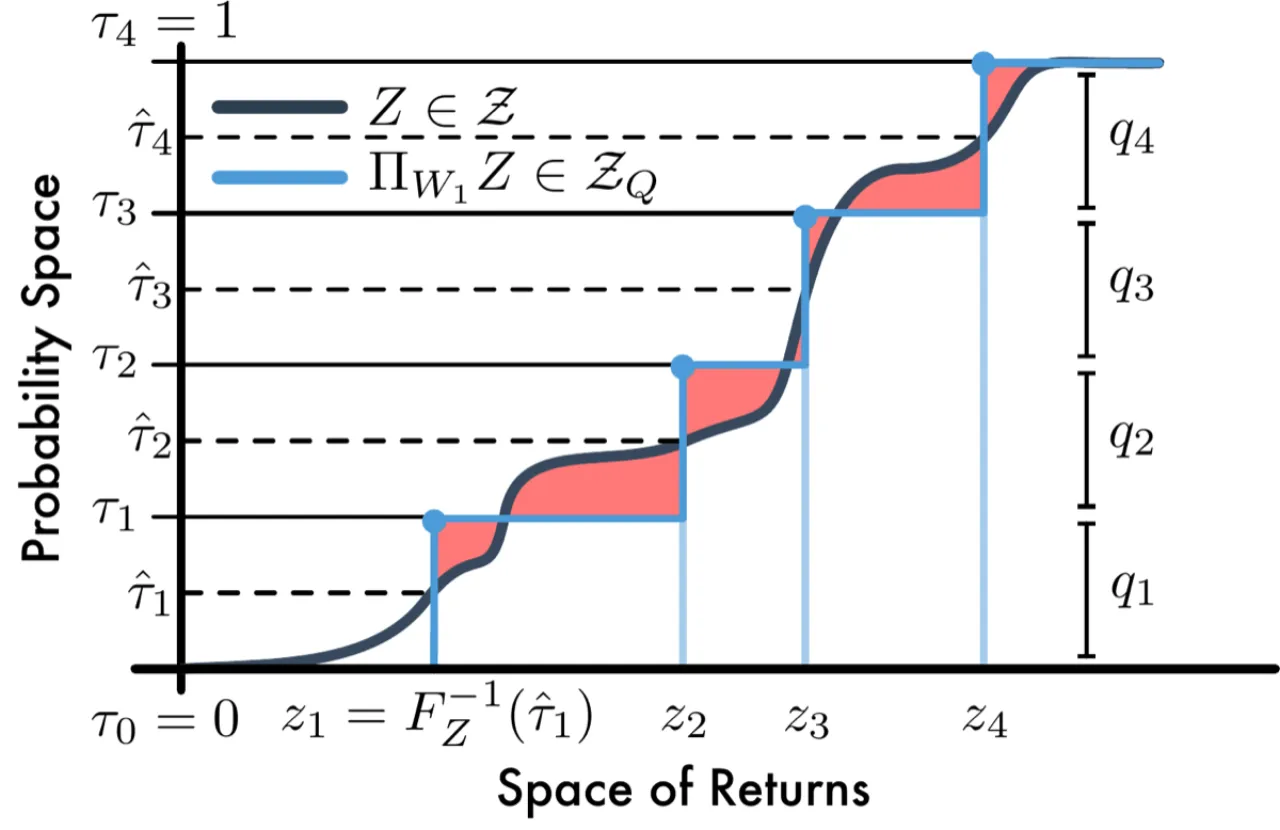
传统强化学习只学习期望回报(value function),而 QR-DQN 将 DQN 扩展为学习完整的回报分布(value distribution):用 N 个等权重的 Dirac 分量参数化分位数分布,通过分位数回归(quantile regression)在 Wasserstein 度量下端到端优化,在理论与实践两方面均弥合了此前 distributional RL 存在的缺口。Classical reinforcement learning learns only the expected return (value function), whereas QR-DQN extends DQN to learn the full return distribution (value distribution): the quantile distribution is parameterized by N equally weighted Dirac components and optimized end-to-end under the Wasserstein metric via quantile regression, closing the gap that previously existed in distributional RL on both the theoretical and the practical side.
传统的 Q-learning 将回报(return)的随机性平均掉,只估计期望值。Bellemare 等人(C51)虽然提出了分布式 Bellman 算子并证明其在 Wasserstein 度量下是收缩的,却因随机梯度无法直接最小化 Wasserstein 损失而被迫退而求其次,使用 KL 散度加上启发式投影,留下了一个理论与算法之间的缺口。Classical Q-learning averages away the randomness of the return and estimates only its expectation. Bellemare et al. (C51) did propose the distributional Bellman operator and prove that it is a contraction under the Wasserstein metric, but because stochastic gradients cannot directly minimize the Wasserstein loss they had to settle for a KL divergence plus a heuristic projection, leaving a gap between the theory and the algorithm.
"This negative result left open the question as to whether it is possible to devise an online distributional reinforcement learning algorithm which takes advantage of the contraction result... In this paper, we answer this question affirmatively."
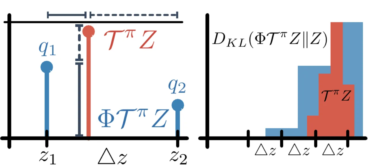
Wasserstein 度量(又称 Earth Mover's Distance,EMD)是分布间的积分概率度量,能够考虑不同结果之间的距离,而 KL 散度在支撑不相交时会产生问题。Lemma 3(来自 C51)已经证明分布式 Bellman 算子 Tπ 在 d̄p(最大化形式的 p-Wasserstein 度量)下是 γ-收缩的:The Wasserstein metric (also known as the Earth Mover's Distance, EMD) is an integral probability metric between distributions that takes the distance between different outcomes into account, whereas the KL divergence breaks down when the supports are disjoint. Lemma 3 (from C51) already proved that the distributional Bellman operator Tπ is a γ-contraction under d̄p (the maximal form of the p-Wasserstein metric):
d̄p(TπZ₁, TπZ₂) ≤ γ · d̄p(Z₁, Z₂)
但随机梯度下降无法直接最小化 Wasserstein 损失(Theorem 1,Bellemare et al. 2017):对于样本经验分布,期望样本损失的最优解与真实 Wasserstein 损失的最优解通常不同。因此,C51 实际用的是 KL 散度,而非 Wasserstein,导致理论与实现脱节。QR-DQN 的核心贡献是找到了一种参数化方式,使得分位数回归可以给出 Wasserstein 的无偏随机梯度。But stochastic gradient descent cannot directly minimize the Wasserstein loss (Theorem 1, Bellemare et al. 2017): for a sample empirical distribution, the minimizer of the expected sample loss generally differs from the minimizer of the true Wasserstein loss. C51 therefore actually uses the KL divergence rather than the Wasserstein metric, which disconnects the theory from the implementation. The core contribution of QR-DQN is a parameterization under which quantile regression yields unbiased stochastic gradients of the Wasserstein loss.
QR-DQN 将 C51 的参数化"转置":C51 用固定位置 + 可变概率,而 QR-DQN 用固定等概率(1/N)+ 可变位置。每个位置对应一个分位数中点,通过分位数回归以无偏随机梯度端到端最小化 1-Wasserstein 距离。QR-DQN "transposes" the C51 parameterization: C51 uses fixed locations with variable probabilities, whereas QR-DQN uses fixed uniform probabilities (1/N) with variable locations. Each location corresponds to one quantile midpoint, and the 1-Wasserstein distance is minimized end-to-end by quantile regression with unbiased stochastic gradients.
对于固定的 N,定义分位数分布为:For a fixed N, the quantile distribution is defined as:
Zθ(x,a) := (1/N) Σi=1..N δθᵢ(x,a)
其中 δz 是在 z 处的 Dirac 质量,θᵢ 是可学习的位置参数。where δz is a Dirac mass at z and the θᵢ are learnable location parameters.
分位数中点为 τ̂ᵢ = (τᵢ₋₁ + τᵢ) / 2,其中 τᵢ = i/N。The quantile midpoints are τ̂ᵢ = (τᵢ₋₁ + τᵢ) / 2, where τᵢ = i/N.
相比 C51,量化分位数分布有三大优势:Compared with C51, the quantile distribution has three major advantages:
对于分位数 τ ∈ [0,1],分位数回归损失是一种非对称凸损失,过高估计以权重 τ 惩罚,过低估计以权重 1-τ 惩罚:For a quantile τ ∈ [0,1], the quantile regression loss is an asymmetric convex loss that penalizes overestimation with weight τ and underestimation with weight 1-τ:
LτQR(θ) = EẐ∼Z[ρτ(Ẑ - θ)],其中 ρτ(u) = u(τ - 𝟙{u<0})LτQR(θ) = EẐ∼Z[ρτ(Ẑ - θ)], where ρτ(u) = u(τ - 𝟙{u<0})
由 Lemma(w1_midpoint)可知,令 θᵢ = F-1Z(τ̂ᵢ) 即可最小化 1-Wasserstein 距离。By the Lemma (w1_midpoint), setting θᵢ = F-1Z(τ̂ᵢ) minimizes the 1-Wasserstein distance.
因此,以下目标函数的最小化等价于最小化 W₁(Z, Zθ):Minimizing the following objective is therefore equivalent to minimizing W₁(Z, Zθ):
Σᵢ EẐ∼Z[ρτ̂ᵢ(Ẑ - θᵢ)]
此损失提供无偏样本梯度,可直接用随机梯度下降优化。This loss provides unbiased sample gradients and can be optimized directly by stochastic gradient descent.
标准分位数回归损失在零点不光滑,可能限制非线性函数近似的性能。论文引入 Quantile Huber Loss:在 [-κ, κ] 区间内用非对称平方损失,超出区间回退到标准分位数损失:The standard quantile regression loss is not smooth at zero, which may limit the performance of non-linear function approximation. The paper introduces the Quantile Huber Loss: an asymmetric squared loss on the interval [-κ, κ] that falls back to the standard quantile loss outside that interval:
ρκτ(u) = |τ - 𝟙{u<0}| · Lκ(u)
其中 Lκ(u) = u²/2 if |u|≤κ, else κ(|u| - κ/2)(Huber 损失)。实验中 κ=1,记为 QR-DQN-1。where Lκ(u) = u²/2 if |u|≤κ, else κ(|u| - κ/2) is the Huber loss. The experiments use κ=1, denoted QR-DQN-1.
论文证明(Proposition),分位数投影 ΠW₁ 与分布式 Bellman 算子 Tπ 的组合在 d̄∞ 下是 γ-收缩的:The paper proves (Proposition) that the composition of the quantile projection ΠW₁ with the distributional Bellman operator Tπ is a γ-contraction under d̄∞:
d̄∞(ΠW₁ Tπ Z₁, ΠW₁ Tπ Z₂) ≤ γ · d̄∞(Z₁, Z₂)
这意味着组合算子存在唯一不动点,算法(及其随机近似)收敛到该不动点,且对所有 p ∈ [1,∞] 收敛。这是 distributional RL 在 Wasserstein 度量下端到端保证的首个实例。This means that the composed operator has a unique fixed point, that the algorithm (and its stochastic approximation) converges to that fixed point, and that convergence holds for all p ∈ [1,∞]. This is the first instance of an end-to-end guarantee for distributional RL under the Wasserstein metric.
QR-DQN 相对 DQN 有三处修改:QR-DQN makes three modifications to DQN:
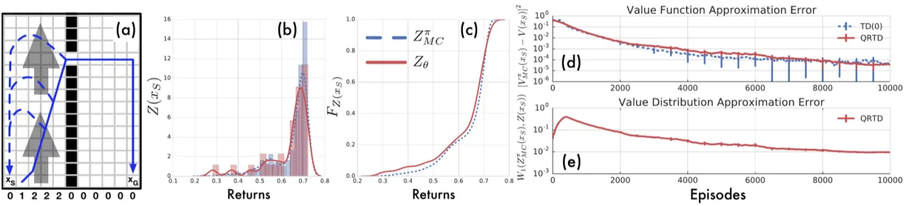
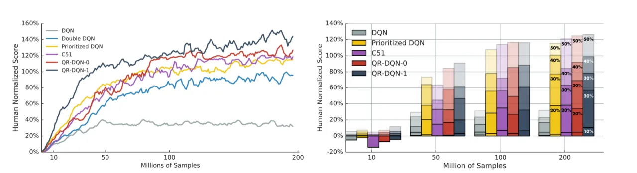
实验分两部分:(1)在经典的两室风格子世界(windy gridworld)上验证 QR-TD 确实学习到真实回报分布;(2)在 57 个 Atari 2600 游戏上对比 DQN、DDQN、Dueling、Prioritized Replay、C51 等 baseline,使用人类归一化得分评估。The experiments come in two parts: (1) a classical two-room windy gridworld verifying that QR-TD really does learn the true return distribution; (2) a comparison against baselines such as DQN, DDQN, Dueling, Prioritized Replay and C51 on 57 Atari 2600 games, evaluated with human-normalized scores.
超参数搜索结果:α = 0.00005,εADAM = 0.01/32,N = 200。以下数据来自论文 Table 1(200 million 训练帧,57 游戏):Hyper-parameter search results: α = 0.00005, εADAM = 0.01/32, N = 200. The figures below are taken from Table 1 of the paper (200 million training frames, 57 games):
| 算法Algorithm | Mean (human-norm.) | Median (human-norm.) | >Human | >DQN |
|---|---|---|---|---|
| DQN | 228% | 79% | 24 | 0 |
| DDQN | 307% | 118% | 33 | 43 |
| Dueling | 373% | 151% | 37 | 50 |
| Prioritized | 434% | 124% | 39 | 48 |
| Pr. Dueling | 592% | 172% | 39 | 44 |
| C51 | 701% | 178% | 40 | 50 |
| QR-DQN-0 (κ=0) | 881% | 199% | 38 | 52 |
| QR-DQN-1 (κ=1) | 915% | 211% | 41 | 54 |
在含随机转移的两室风格子世界中,以 1K Monte-Carlo rollout 估计真实分布,运行 TD 和 QR-TD 各 10K episodes(N=32,学习率 α=0.1)。结果显示 QR-TD 正确收敛并最小化了与 MC 估计之间的 1-Wasserstein 距离,而标准 TD 仅收敛均值。In a two-room windy gridworld with stochastic transitions, the true distribution is estimated with 1K Monte-Carlo rollouts, and TD and QR-TD are each run for 10K episodes (N=32, learning rate α=0.1). The results show that QR-TD converges correctly and minimizes the 1-Wasserstein distance to the MC estimate, while standard TD converges only in the mean.
论文在 online 评估协议下得出三个关键发现:Under the online evaluation protocol the paper draws three key findings:
QR-DQN 学习了完整的回报分布,但动作选择仍依赖期望值:a* = argmaxa' Ez∼Z(x',a')[z]。论文明确指出这是当前设计的限制,并提出更丰富的策略类——基于完整分布进行风险敏感决策(risk-sensitive decision making)——是重要的未来方向。QR-DQN learns the full return distribution, but action selection still relies on the expectation: a* = argmaxa' Ez∼Z(x',a')[z]. The paper explicitly notes this as a limitation of the current design and proposes richer policy classes — risk-sensitive decision making based on the full distribution — as an important future direction.
论文测试的是"纯"QR-DQN,未叠加 Dueling architecture、Prioritized Replay 等近年对 DQN 的改进。论文明确指出:"A natural next step would be to combine QR-DQN with the non-distributional methods found in Table 1。"(QR-DQN 在 54 个游戏上超过 DQN,但未必在所有改进组合上达到最优。)The paper tests "pure" QR-DQN, without stacking recent DQN improvements such as the Dueling architecture or Prioritized Replay. It states explicitly: "A natural next step would be to combine QR-DQN with the non-distributional methods found in Table 1." (QR-DQN beats DQN on 54 games, but is not necessarily optimal in combination with every improvement.)
论文证明了 ΠW₁ Tπ 在 d̄∞ 下是收缩的,但明确指出 "the contraction property does not directly hold for p < ∞"(详见附录 Lemma)。这意味着理论保证最强在 ∞-Wasserstein 意义下成立,1-Wasserstein 下的收敛性需要额外论证。The paper proves that ΠW₁ Tπ is a contraction under d̄∞, but notes explicitly that "the contraction property does not directly hold for p < ∞" (see the appendix Lemma). This means the theoretical guarantee is strongest in the ∞-Wasserstein sense, and convergence under 1-Wasserstein requires additional argument.
QR-DQN 将输出层从 |A| 扩展到 |A|×N,且损失对所有 N² 对 (θᵢ, TΘⱼ) 求和,计算与内存成本均随 N² 增长。最优 N=200 是通过在五个训练游戏上超参数搜索得到的,增加了调参代价。QR-DQN widens the output layer from |A| to |A|×N, and the loss sums over all N² pairs (θᵢ, TΘⱼ), so both computation and memory cost grow with N². The optimal N=200 was obtained by a hyper-parameter search over five training games, which adds to the tuning cost.