Diffusion Model Guided Sampling with Pixel-Wise Aleatoric Uncertainty Estimation
逐像素不确定性估计引导扩散模型采样,无需额外训练Pixel-wise uncertainty estimation guides diffusion model sampling, no extra training required
Michele De Vita & Vasileios Belagiannis · Friedrich-Alexander-Universität Erlangen-Nürnberg
扩散模型能够生成高质量图像,但缺乏对生成样本质量的定量评估手段。本文提出一种无需训练的方法,在采样每一步估计逐像素的 aleatoric uncertainty,并将其作为引导信号,在 ImageNet 和 CIFAR-10 上以更少的函数评估次数(NFEs)改善 FID,同时可用于过滤低质量样本。Diffusion models can generate high-quality images, but lack a quantitative means of assessing the quality of the generated samples. This paper proposes a training-free method that estimates pixel-wise aleatoric uncertainty at every sampling step and uses it as a guidance signal, improving FID on ImageNet and CIFAR-10 with fewer function evaluations (NFEs), while also serving to filter out low-quality samples.
扩散模型在图像生成领域取得了显著进展,但生成样本的质量良莠不齐,且缺乏量化评估手段。
在安全敏感应用(如医学影像、自动驾驶)中,理解并量化生成样本的不确定性至关重要。
现有不确定性方法(如 MC Dropout、集成方法)计算代价高昂,或对模型结构有侵入性要求;
唯一面向扩散模型的逐像素方法 BayesDiff 需要显著的额外计算开销,且未将不确定性用于引导生成。Diffusion models have made remarkable progress in image generation, yet the quality of generated samples varies widely and quantitative assessment is lacking. In safety-critical applications such as medical imaging and autonomous driving, understanding and quantifying the uncertainty of generated samples is essential. Existing uncertainty methods such as MC Dropout and ensembles are computationally expensive or make intrusive demands on the model architecture; BayesDiff, the only pixel-wise method aimed at diffusion models, requires substantial extra computation and does not use the uncertainty to guide generation.
"understanding and quantifying the uncertainty associated with generated samples is crucial for ensuring the quality of the data"
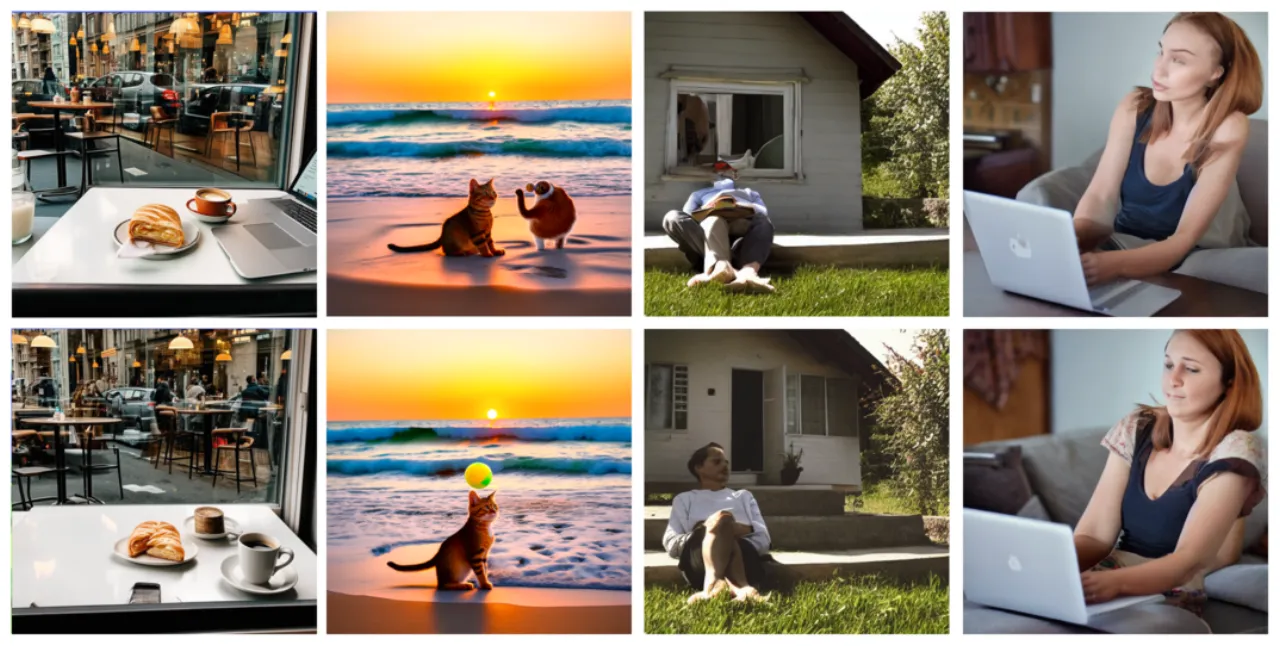
图1: Stable Diffusion 3 和 1.5 在有无不确定性引导下的生成对比。
上行为标准生成,下行为 uncertainty-guided 生成结果,伪影更少、细节更忠实。Figure 1: Comparison of generation with and without uncertainty guidance for Stable Diffusion 3 and 1.5. The top row is standard generation, the bottom row is uncertainty-guided generation, with fewer artifacts and more faithful detail.
20本方法 NFEs(函数评估次数)NFEs (number of function evaluations) of our method
130BayesDiff 所需 NFEs(6.5×)NFEs required by BayesDiff (6.5×)
−1 FIDuncertainty guidance 带来的平均改善average improvement brought by uncertainty guidance
Training-free无需修改或重新训练模型no model modification or retraining required
02方法 MethodMethod
方法核心是:在每个采样步骤 t,先从当前带噪样本 Xt 近似预测干净图像 X̂0,
再利用扩散模型正向过程的加噪分布对 X̂0 进行 M 次微扰,得到多个噪声变体,
最终以这些变体预测分数的方差作为逐像素 aleatoric uncertainty 的代理估计。
所得不确定性图可用于两个下游任务:过滤低质量样本(uncertainty filtering),以及引导采样(uncertainty guided sampling)。The core of the method: at each sampling step t, first approximate the clean image X̂0 from the current noisy sample Xt; then perturb X̂0M times with the noising distribution of the diffusion forward process to obtain multiple noisy variants; finally take the variance of the scores predicted for these variants as a proxy estimate of the pixel-wise aleatoric uncertainty. The resulting uncertainty map serves two downstream tasks: filtering low-quality samples (uncertainty filtering), and guiding sampling (uncertainty guided sampling).
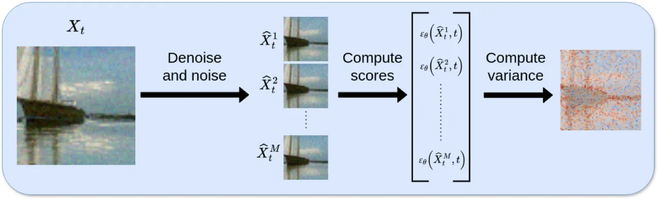
图2:不确定性估计算法示意(时间步 t)。
Step 1:由 Xt 和噪声预测网络 εθ 近似 X̂0;
Step 2:从加噪分布 q(X̂ti | X̂0) 采样 M 个变体;
Step 3:计算各变体的预测分数方差,得到不确定性图 Ut。Figure 2: Illustration of the uncertainty estimation algorithm (time step t). Step 1: approximate X̂0 from Xt and the noise prediction network εθ; Step 2: sample M variants from the noising distribution q(X̂ti | X̂0); Step 3: compute the variance of the predicted scores over the variants to obtain the uncertainty map Ut.
首先,从当前步 Xt 近似重建干净图像:First, approximately reconstruct the clean image from the current step Xt:
X̂0 = (Xt − √(1−ᾱt) εθ(Xt, t)) / √ᾱt
接着对 X̂0 施加扩散正向加噪,得到 M 个噪声变体 {X̂ti},
对每个变体运行去噪网络得到分数估计 Et,不确定性图定义为:Next, apply the diffusion forward noising to X̂0 to obtain M noisy variants {X̂ti}, run the denoising network on each variant to obtain the score estimates Et, and define the uncertainty map as:
Ut = diag((Et − Ēt)T(Et − Ēt))
理论上,该估计近似于加噪分布的 Fisher information(对数似然的二阶导数的负期望),
从而为不确定性估计赋予了信息几何学意义。In theory this estimate approximates the Fisher information of the noising distribution (the negative expectation of the second derivative of the log-likelihood), which endows the uncertainty estimate with an information-geometric meaning.
利用不确定性图对分数估计进行梯度修正:高不确定性像素(超过分位阈值 p 的区域)
通过梯度更新 ∂Ut/∂εt 引导噪声预测修正,更新强度由超参数 λ 控制:The uncertainty map is used to apply a gradient correction to the score estimate: pixels of high uncertainty (regions above the percentile threshold p) drive a correction of the noise prediction through the gradient update ∂Ut/∂εt, with the update strength controlled by the hyperparameter λ:
ε̂t = εt + λ · (I[Ut > p] · ∂Ut/∂εt)
该操作在每个采样步骤插入,鼓励模型降低高不确定性区域的分数估计方差,从而产生质量更高的样本。This operation is inserted at every sampling step, encouraging the model to reduce the variance of the score estimates in high-uncertainty regions and thereby produce samples of higher quality.
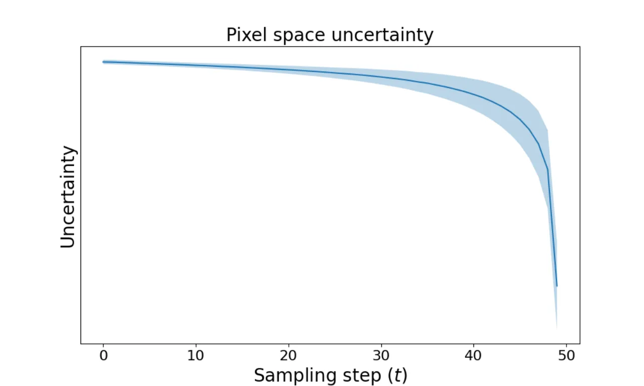
图3:像素空间不确定性随采样进程的变化曲线。
以 ADM 在 60,000 张 ImageNet 样本上统计,蓝线为平均值,阴影为标准差。
可见不确定性在最后去噪阶段(约 75–90% 进程处)急剧升高,说明最终几步对生成质量影响最大。Figure 3: Pixel-space uncertainty over the course of sampling. Statistics computed with ADM over 60,000 ImageNet samples; the blue line is the mean, the shading the standard deviation. Uncertainty rises sharply in the final denoising stage (around 75–90% of the trajectory), showing that the last few steps matter most for generation quality.
03实验 ExperimentsExperiments
在 ImageNet(64×64、128×128、256×256、512×512)和 CIFAR-10 上评估,
使用模型:ADM(ImageNet64/128)、U-ViT(ImageNet256/512)、DDPM(CIFAR-10)。
评估指标:FID(图像质量)、AUSE(不确定性校准,越低越好)、AURG(越高越好)。Evaluation on ImageNet (64×64, 128×128, 256×256, 512×512) and CIFAR-10, with the models ADM (ImageNet64/128), U-ViT (ImageNet256/512) and DDPM (CIFAR-10). Metrics: FID (image quality), AUSE (uncertainty calibration, lower is better) and AURG (higher is better).
从 60,000 张生成图像中按不确定性排序,过滤高不确定性样本后重新计算 FID。Generated images are ranked by uncertainty among 60,000 samples, and FID is recomputed after filtering out the high-uncertainty ones.
模型Model
数据集Dataset
Random(基线)Random (baseline)
Ours
BayesDiff
MC-Dropout
ADM
ImageNet64
3.289
3.254
—
3.268
ADM
ImageNet128
8.21
7.88
8.45
—
ADM w/2-DPM
ImageNet128
8.50
8.48
9.67
—
U-ViT
ImageNet256
7.88
7.80
6.81
—
U-ViT
ImageNet512
16.47
16.37
16.87
—
DDPM
CIFAR-10
13.494
13.416
—
13.435
注: 在 ImageNet256 上 BayesDiff 取得了更好的 FID(6.81 vs 7.80),本文方法略逊一筹,
但本文方法仅需 20 NFEs,而 BayesDiff 需要 130 NFEs(高出约 6.5×)。Note: On ImageNet256 BayesDiff attains a better FID (6.81 vs 7.80) and this method falls slightly behind, but this method needs only 20 NFEs whereas BayesDiff requires 130 NFEs (about 6.5× more).
在标准采样流程中插入不确定性引导更新,生成 10,000 张图像后比较 FID。The uncertainty guidance update is inserted into the standard sampling procedure and FID is compared after generating 10,000 images.
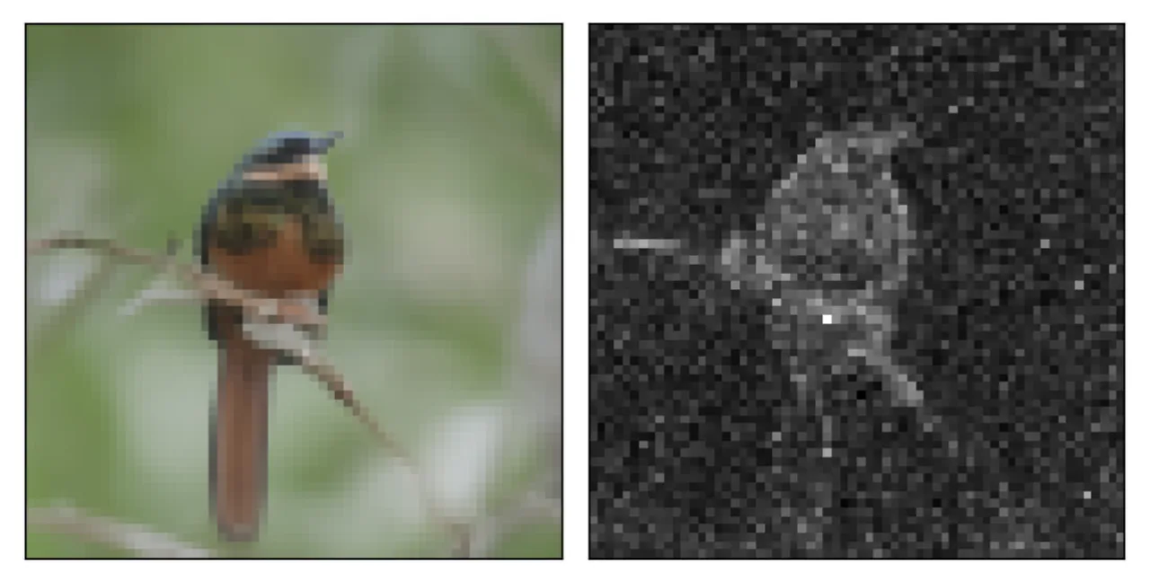
图4:逐像素不确定性图示例(推断噪声方案)。
高不确定性区域(亮色)集中在图像的边缘、纹理复杂区域,与感知质量问题高度吻合。Figure 4: Examples of pixel-wise uncertainty maps (inferred noise schedule). The high-uncertainty regions (bright areas) concentrate on image edges and texturally complex areas, matching perceptual quality problems closely.
消融实验Ablation studies
作者对分位阈值 p(percentile)和引导强度 λ 进行了超参数扫描。
结果表明:p 在 75–90 分位附近、λ 在较小范围内时效果最稳定。
M(扰动次数)的选择在计算效率与校准精度之间存在权衡:
更大的 M 在 CIFAR-10 和 ImageNet64 上带来边际收益,但增加了计算开销。The authors sweep the percentile threshold p (percentile) and the guidance strength λ. The results show that p around the 75–90 percentile and λ within a small range are the most stable. The choice of M (number of perturbations) trades computational efficiency against calibration accuracy: a larger M brings marginal gains on CIFAR-10 and ImageNet64, but increases the computational cost.
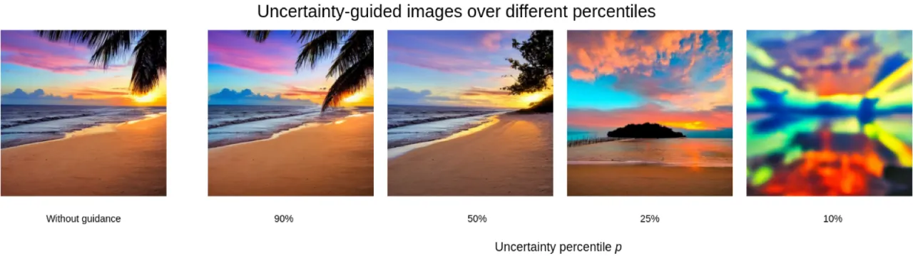
图5:百分位阈值 p 的消融结果。
不同数据集上随着 p 的变化,FID 呈现先下降后上升的趋势,
说明只聚焦于最高不确定性的少数像素时效果最好。Figure 5: Ablation on the percentile threshold p. Across datasets, FID first falls and then rises as p varies, showing that focusing on only the few most uncertain pixels works best.
04局限性 LimitationsLimitations
说明: 本文没有设置独立的 Limitations 小节。以下局限性部分为作者在实验讨论中明确提及的已知不足(stated),部分为从方法设计推断(inferred)。Note: The paper has no separate Limitations section. Some of the limitations below are shortcomings the authors explicitly acknowledge in their experimental discussion (stated), others are inferred from the method design (inferred).
在 ImageNet256 上被 BayesDiff 超越(stated)Outperformed by BayesDiff on ImageNet256 (stated)
在 ImageNet256 的不确定性过滤实验中,本文方法的 FID 为 7.80,而 BayesDiff 达到 6.81——低于本文方法。
作者在实验结果中明确列出了这一数据,并未回避。这表明在较大分辨率的过滤任务上,本文方法尚有提升空间。In the uncertainty filtering experiment on ImageNet256, this method reaches an FID of 7.80 while BayesDiff reaches 6.81 — lower than this method. The authors list this figure explicitly in their results and do not avoid it. It indicates that on filtering tasks at larger resolutions this method still has room to improve.
性能依赖超参数选择(inferred)Performance depends on hyperparameter choice (inferred)
方法引入两个超参数:分位阈值 p(决定哪些像素被引导)和更新强度 λ。
消融实验表明不同数据集/模型下最优值不同,需要在实际部署时针对具体设置进行调整,
降低了"开箱即用"的便捷性。The method introduces two hyperparameters: the percentile threshold p (which decides which pixels are guided) and the update strength λ. The ablations show that the optimum differs across datasets and models, so it has to be tuned for the specific setting at deployment time, which reduces its out-of-the-box convenience.
引导仅作用于高不确定性像素(inferred)Guidance acts only on high-uncertainty pixels (inferred)
indicator function I[Ut > p] 限定了梯度更新仅在超过阈值的像素上生效,
对于不确定性分布较均匀(全图不确定性相近)的样本,引导效果可能有限。The indicator function I[Ut > p] restricts the gradient update to pixels above the threshold, so for samples whose uncertainty is fairly uniformly distributed (similar uncertainty over the whole image) the guidance may have limited effect.