通过贝叶斯推断估计扩散模型生成图像的逐像素不确定性Estimating pixel-wise uncertainty of diffusion-generated images via Bayesian inference
Siqi Kou · Lei Gan · Dequan Wang · Chongxuan Li · Zhijie Deng
扩散模型在图像生成上表现优异,但仍会产生质量低劣的样本,而现有方法难以在单样本层面识别它们。BayesDiff 将 Bayesian inference 引入预训练扩散模型,推导出 uncertainty iteration 原理,估计每个像素的不确定性,从而实现低质量图像过滤、多样性增强与 artifact 纠正。Diffusion models excel at image generation, yet they still produce low-quality samples that existing methods can hardly identify at the level of an individual sample. BayesDiff introduces Bayesian inference into pretrained diffusion models and derives an uncertainty iteration principle that estimates the uncertainty of every pixel, thereby enabling low-quality image filtering, diversity augmentation and artifact correction.
扩散模型(diffusion models)在图像生成领域取得了令人瞩目的成就,但其生成过程并不总是可靠:即使是同一个模型,也会产生质量参差不齐的样本,包括语义混乱、artifact 明显或与文本 prompt 不符的图像。现有评估指标(如 FID、Inception Score)只能衡量整体分布质量,无法针对单张图像做出判断,这使得低质量图像的识别与过滤几乎无从下手。Diffusion models have achieved remarkable results in image generation, but their generative process is not always reliable: even one and the same model produces samples of uneven quality, including images with semantic confusion, conspicuous artifacts, or a mismatch with the text prompt. Existing evaluation metrics such as FID and Inception Score only measure the quality of the overall distribution and cannot make a judgement about a single image, which leaves the identification and filtering of low-quality images almost without a handle.
"Bayesian uncertainty has long been used to identify data far from the manifold of training samples — the posterior delivers low uncertainty for training-like data and high uncertainty for others."
作者将 Bayesian uncertainty 的这一特性迁移到扩散模型的生成过程中:如果一张生成图像的像素分布偏离训练数据的流形,则该像素对应的不确定性应当更高。基于这一直觉,BayesDiff 建立了一套从 Bayesian inference 出发、跟踪整个反向扩散链(reverse diffusion chain)中不确定性传播的理论框架。The authors transfer this property of Bayesian uncertainty to the generative process of diffusion models: if the pixel distribution of a generated image deviates from the manifold of the training data, the uncertainty of that pixel should be higher. Based on this intuition, BayesDiff builds a theoretical framework that starts from Bayesian inference and tracks the propagation of uncertainty throughout the entire reverse diffusion chain.
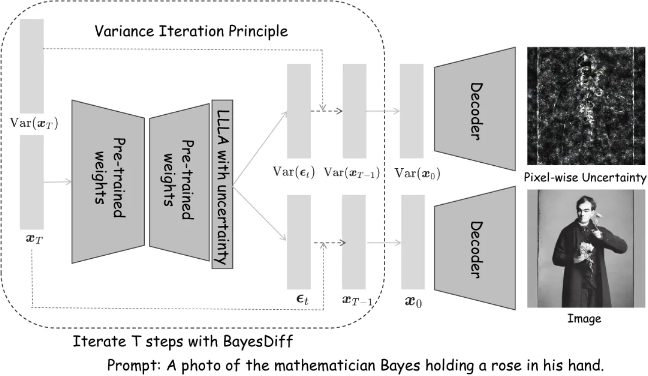
图 1:BayesDiff 总览。在标准 DDPM/DDIM 的每一个去噪步骤中,BayesDiff 额外维护一个逐像素 variance 估计,并通过 uncertainty iteration 原理将其从第 T 步传播到第 0 步,最终得到与生成图像同尺寸的不确定性图(uncertainty map)。Figure 1: Overview of BayesDiff. At every denoising step of standard DDPM/DDIM, BayesDiff additionally maintains a pixel-wise variance estimate and propagates it from step T down to step 0 through the uncertainty iteration principle, finally yielding an uncertainty map of the same size as the generated image.
Pixel-wise不确定性集中于语义关键区域(眼睛、轮廓等)Uncertainty concentrates on semantically critical regions (eyes, contours, etc.)
02方法 (Method)Method
BayesDiff 在不改动预训练扩散模型权重的前提下,通过两个核心组件实现逐像素不确定性估计:(1)Last-Layer Laplace Approximation (LLLA) 将噪声预测网络的最后一层替换为贝叶斯线性层,以高效方式获得像素级方差预测;(2)Uncertainty Iteration Principle 推导出在整个反向扩散链中方差如何逐步传播的解析公式。Without modifying the weights of the pretrained diffusion model, BayesDiff performs pixel-wise uncertainty estimation through two core components: (1) the Last-Layer Laplace Approximation (LLLA) replaces the last layer of the noise-prediction network with a Bayesian linear layer, obtaining pixel-level variance predictions in an efficient manner; (2) the Uncertainty Iteration Principle derives an analytical formula for how the variance propagates step by step along the whole reverse diffusion chain.
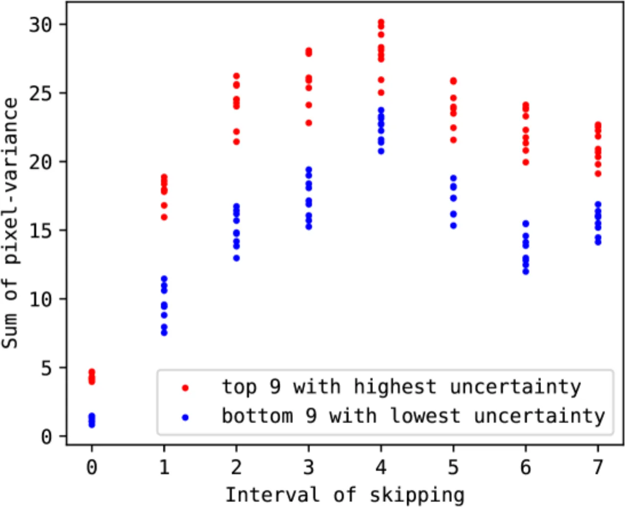
图 2:BayesDiff-Skip 可靠性研究。仅在选定的去噪步骤上计算不确定性,在 5× 加速的同时仍能与全步骤版本保持高度一致的样本质量排序。Figure 2: Reliability study of BayesDiff-Skip. Computing uncertainty only at selected denoising steps still preserves a sample-quality ranking highly consistent with the full-step version, while achieving a 5× speedup.
Last-Layer Laplace Approximation (LLLA)
标准 Laplace approximation 对完整神经网络的 Hessian 进行近似,计算代价极高。LLLA 只对最后一层(线性输出层)应用 Laplace 近似,将后验近似为 Gaussian:参数均值为预训练权重,协方差由 Generalized Gauss-Newton (GGN) 矩阵给出。推理时,对最后一层权重 marginalize 后可得到像素级输出分布,从而获得逐像素的预测方差 Var(ε̂_t)。此步骤只需在训练集上一次性计算 GGN 矩阵,与扩散模型的生成步骤解耦。The standard Laplace approximation approximates the Hessian of the full neural network, which is computationally prohibitive. LLLA applies the Laplace approximation only to the last layer (the linear output layer) and approximates the posterior as a Gaussian: the parameter mean is the pretrained weight and the covariance is given by the Generalized Gauss-Newton (GGN) matrix. At inference time, marginalizing over the last-layer weights yields a pixel-level output distribution and hence the pixel-wise predictive variance Var(ε̂_t). This step only requires a one-off computation of the GGN matrix on the training set and is decoupled from the sampling steps of the diffusion model.
Uncertainty Iteration Principle
在标准 DDPM/DDIM 框架中,x_{t-1} 由 x_t 和预测噪声 ε̂_t 通过确定性或随机公式计算而来。BayesDiff 将此过程视为一个随机变量的线性传播,推导出方差传播的解析公式(论文 Equation 8):In the standard DDPM/DDIM framework, x_{t-1} is computed from x_t and the predicted noise ε̂_t through a deterministic or stochastic formula. BayesDiff regards this process as the linear propagation of a random variable and derives an analytical formula for variance propagation (Equation 8 of the paper):
其中 Cov(x_t, ε_t) 通过 Monte Carlo 采样估计(Equation 11),整个传播过程从 t=T 运行到 t=0,最终得到生成图像 x_0 的逐像素 variance 图。Here Cov(x_t, ε_t) is estimated by Monte Carlo sampling (Equation 11); the whole propagation runs from t=T down to t=0, finally yielding the pixel-wise variance map of the generated image x_0.
完整算法在每个去噪步骤都需要额外的 Monte Carlo 采样来估计协方差,计算开销较大(超过 S>10 次额外模型前向)。BayesDiff-Skip 只在预先选定的若干关键步骤上执行不确定性计算,其余步骤跳过,从而实现"5× reduction in running time",同时保持对样本质量排序的高度一致性(如图 2 所示)。At every denoising step the full algorithm needs extra Monte Carlo sampling to estimate the covariance, which is computationally expensive (more than S>10 extra model forward passes). BayesDiff-Skip computes uncertainty only at a few pre-selected key steps and skips the rest, thereby achieving a "5× reduction in running time" while keeping the ranking of sample quality highly consistent (as shown in Figure 2).
03实验 (Experiments)Experiments
实验在 ImageNet 256×256(U-ViT)、ImageNet 128×128(ADM,DDIM/DPM-Solver)和 CELEBA 等数据集上进行,覆盖条件生成与无条件生成场景;文本到图像实验使用 Stable Diffusion v1.4。评估指标包括 FID、Precision、Recall。核心任务分为三类:低质量图像过滤、多样性增强(diversity augmentation)与 artifact 纠正。Experiments are conducted on ImageNet 256×256 (U-ViT), ImageNet 128×128 (ADM, with DDIM/DPM-Solver) and CELEBA, covering both conditional and unconditional generation; the text-to-image experiments use Stable Diffusion v1.4. The evaluation metrics include FID, Precision and Recall. The core tasks fall into three categories: low-quality image filtering, diversity augmentation and artifact correction.
低质量图像过滤(Filtering)Low-Quality Image Filtering
从 50,000 张生成图像中,按不确定性排序,过滤掉 top 16% 高不确定性样本,再评估剩余图像的 FID 与 Precision。From 50,000 generated images, samples are ranked by uncertainty, the top 16% with the highest uncertainty are filtered out, and FID and Precision are then evaluated on the remaining images.
模型 / 数据集Model / Dataset
采样器Sampler
FID(过滤前)FID (before filtering)
FID(过滤后)FID (after filtering)
Precision(前→后)Precision (before → after)
U-ViT ImageNet 256
DDIM
7.24±0.02
6.81
0.698 → 0.705
ADM ImageNet 128
DDIM
8.68±0.04
8.48
0.661 → 0.665
ADM ImageNet 128
DPM-Solver
9.77±0.03
9.67
0.657 → 0.659
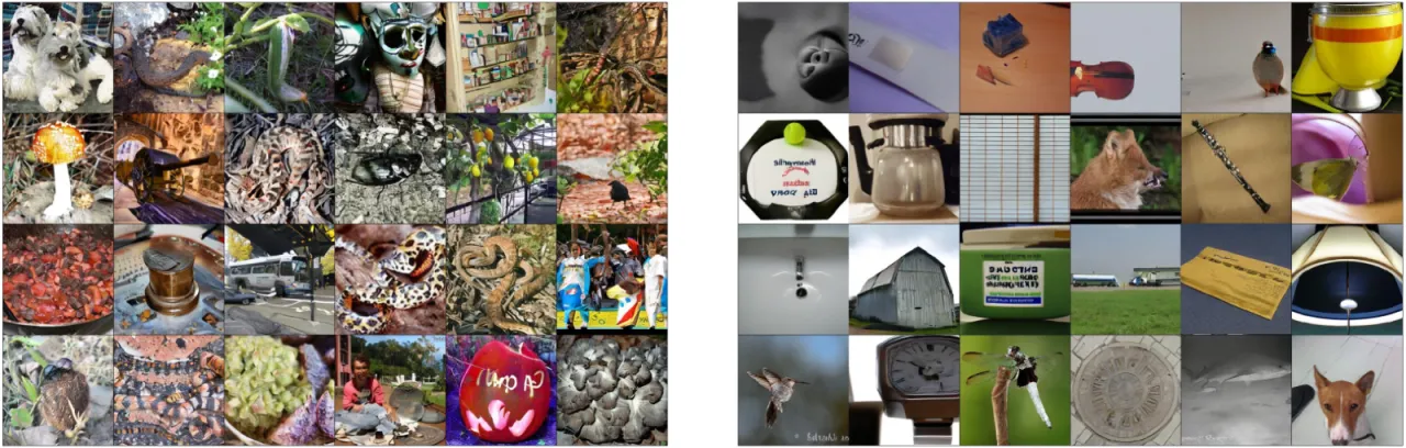
图 3:U-ViT 在 ImageNet 256×256 上生成的最高(上行)与最低(下行)不确定性样本。高不确定性图像明显存在语义混乱或结构失真,而低不确定性图像质量明显更好。Figure 3: Samples with the highest (top row) and lowest (bottom row) uncertainty generated by U-ViT on ImageNet 256×256. The high-uncertainty images clearly exhibit semantic confusion or structural distortion, whereas the low-uncertainty images are markedly better in quality.图 4:Stable Diffusion 上的不确定性对比(512×512)。高不确定性区域(暖色)精确对应图像中的失真或语义错误区域,如错误的手指数量、模糊的面部特征等。Figure 4: Uncertainty comparison on Stable Diffusion (512×512). Regions of high uncertainty (warm colors) correspond precisely to the distorted or semantically wrong areas of the image, such as an incorrect number of fingers or blurred facial features.
文本到图像:多样性增强与 Artifact 纠正Text-to-Image: Diversity Augmentation and Artifact Correction
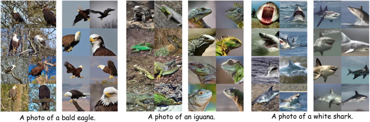
在 t=40 时对高不确定性区域重采样(resampling from estimated distributions),可在保留低不确定性区域结构的前提下产生多样化变体。对于 artifact 明显的失败样本,同样通过局部重采样实现纠正,使输出与 prompt 语义一致。Resampling the high-uncertainty regions at t=40 (resampling from estimated distributions) produces diverse variants while preserving the structure of the low-uncertainty regions. For failure cases with conspicuous artifacts, local resampling likewise achieves a correction that makes the output semantically consistent with the prompt.
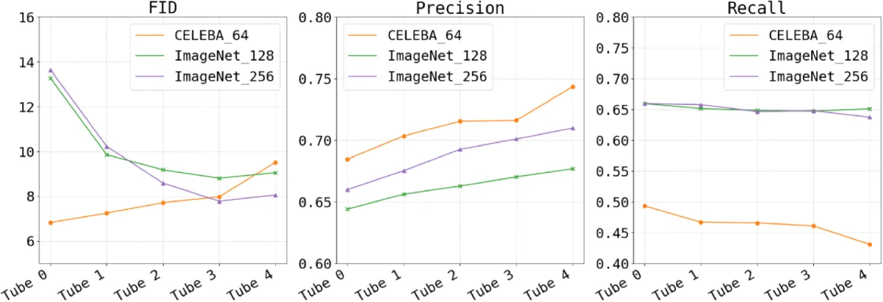
图 5:在不同数据集上,不确定性与 FID、Precision、Recall 的相关性分析。高不确定性样本对应更高的 Recall(多样性),低不确定性样本具有更高的 Precision(保真度),且不确定性分布近似正态。Figure 5: Correlation analysis between uncertainty and FID, Precision and Recall across datasets. High-uncertainty samples correspond to higher Recall (diversity), low-uncertainty samples have higher Precision (fidelity), and the uncertainty distribution is approximately normal.
语义可视化与消融实验Semantic Visualization and Ablation Studies
像素级不确定性图揭示了有意义的语义结构:在 CELEBA 人脸数据集上,不确定性集中于眼睛、鼻子、嘴巴等面部特征;在 Stable Diffusion 输出中,不确定性聚集于物体轮廓。消融实验验证了 LLLA 比全参数 Laplace 更高效且性能相当,以及 BayesDiff-Skip 的步骤选择策略的鲁棒性。The pixel-level uncertainty maps reveal meaningful semantic structure: on the CELEBA face dataset, uncertainty concentrates on facial features such as the eyes, nose and mouth; in Stable Diffusion outputs, it gathers along object contours. The ablation studies verify that LLLA is more efficient than full-parameter Laplace at comparable performance, and that the step-selection strategy of BayesDiff-Skip is robust.
04局限性 (Limitations)Limitations
注: 以下局限性部分来自作者在论文中的明确说明,部分为方法设计中的固有约束。Note: Some of the limitations below are stated explicitly by the authors in the paper; others are inherent constraints of the method design.
计算开销较高High computational overhead
基础算法在每个去噪步骤需要超过 S>10 次额外的模型前向传播用于 Monte Carlo 协方差估计,整体计算量显著高于标准扩散采样。BayesDiff-Skip 虽然实现了 5× 加速,但仍需额外开销,在大分辨率或实时生成场景中仍受限。At every denoising step the basic algorithm requires more than S>10 extra model forward passes for Monte Carlo covariance estimation, so its overall cost is substantially higher than standard diffusion sampling. Although BayesDiff-Skip attains a 5× speedup, extra overhead remains, which is still limiting at high resolution or in real-time generation scenarios.
Gaussian 近似假设的局限Limitations of the Gaussian approximation assumption
方法假设 x_t 在每个时间步近似服从正态分布,并以估计的均值和方差表征其分布。这一假设在早期去噪阶段(噪声较多时)较为合理,但在后期阶段(x_t 已接近真实图像分布)可能存在较大偏差。The method assumes that x_t approximately follows a normal distribution at every timestep and characterizes that distribution by the estimated mean and variance. This assumption is reasonable in the early denoising stages, when noise dominates, but may deviate considerably in the later stages, when x_t is already close to the real image distribution.
LLLA 和方差传播均采用对角协方差假设,忽略了不同像素之间的空间相关性。这意味着方法无法建模大范围结构性不一致,而仅能捕获逐像素的独立不确定性。Both LLLA and the variance propagation adopt a diagonal covariance assumption, ignoring the spatial correlation between different pixels. This means the method cannot model large-scale structural inconsistency and captures only independent pixel-wise uncertainty.
仅近似最后一层的不确定性Only the uncertainty of the last layer is approximated
Last-Layer Laplace Approximation 仅对网络最后一线性层应用贝叶斯处理,中间层的参数不确定性被完全忽略。这是一种权衡计算效率的近似,可能低估总体模型不确定性。The Last-Layer Laplace Approximation applies Bayesian treatment only to the last linear layer of the network, and the parameter uncertainty of the intermediate layers is ignored entirely. This is an approximation that trades against computational efficiency and may underestimate the overall model uncertainty.
依赖训练数据的分布特性Dependence on the distributional properties of the training data
不确定性估计的质量依赖于 GGN 矩阵的准确计算,而 GGN 矩阵由训练数据决定。对于 out-of-distribution 的生成 prompt,或当测试时分布与训练分布差异较大时,不确定性估计的可靠性尚不明确。The quality of the uncertainty estimate depends on an accurate computation of the GGN matrix, which is in turn determined by the training data. For out-of-distribution generation prompts, or when the test-time distribution differs substantially from the training distribution, the reliability of the uncertainty estimate remains unclear.